Mr Kidman's Classroom



Revise the key ideas
Computational thinking
- Decomposition — A quiz application can separate loading questions, collecting answers, marking and reporting scores. Each part can be developed and tested, then connected. Define the interfaces and required information so the pieces solve the original problem together.
- Abstraction — A route model may keep locations and connections while omitting building colours. What is relevant depends on the purpose: accessibility planning may need slope and step information. Abstraction simplifies a model without removing information essential to the problem.
- Algorithmic thinking — An algorithm gives an unambiguous procedure, including decisions and repetition when necessary. Specify how valid input becomes output and when processing stops. A wish such as 'find the best score' needs an actual method, not just a restatement of the goal.
Designing and tracing
- Inputs processes outputs — For a ticket cost, inputs could be ticket count and unit price; processing multiplies them; output is total cost. Include constraints such as a non-negative count. A clear specification helps distinguish correct behaviour from merely producing some output.
- Structure diagrams — A structure diagram breaks a task into modules, such as booking, payment and confirmation. Lines show their structural connections. It is different from a flowchart, which represents the order and decisions within a procedure.
- Pseudocode and flowcharts — Pseudocode expresses operations in a readable programming-like form. Flowcharts use start/end symbols, input/output parallelograms, process rectangles and decision diamonds with labelled branches. Directional arrows must make the next step and any loop unambiguous.
- Selection and iteration — A decision chooses a path based on a condition. A loop repeats a body while or until a condition, or for a specified count. Test whether the condition is checked before or after the body: that affects whether the body can run zero times.
- Trace tables — A trace table tracks variables, conditions and outputs in execution order. For total = 0 and adding 2, 4, 6, successive totals are 2, 6, 12. Follow the actual assignments rather than guessing from the intended purpose.
Python accumulator trace total = 0 for value in [2, 4, 6]: total = total + value print(total)Outputs 2, then 6, then 12. Trace total after each assignment.
- Tracing a branch — If score = 7 and the condition score >= 10 is false, execute the alternative branch. A later instruction outside the branch still executes. Record outputs exactly as produced, including when no output occurs.
- Correcting algorithms — An algorithm starting maximum at 0 fails on a non-empty list of all negative numbers. Initialising it to the first element and then comparing remaining items fixes that case. Explain the cause, corrected step and retest; do not change code only to match one example.
- Refining requirements — Clarify whether a list can be empty, whether equal values are allowed and how a search reports failure. Check loop limits so each intended element is processed once. An algorithm that works only for an unstated narrow example is not a complete solution.
Searching
- Linear search — Linear search compares the target with each item in turn. It works on unsorted data and can stop when a match is found. If no match exists, it may inspect the whole list. Keep the returned position or failure value separate from the target value.
Python linear search def linear_search(values, target): for index in range(len(values)): if values[index] == target: return index return -1 print(linear_search([9, 3, 7, 1], 7))Outputs 2. Return -1 is the explicitly chosen not-found result.
- Linear-search example — To find 7 in [9, 3, 7, 1], compare 9 then 3 then 7: three comparisons find the match at zero-based index 2. If searching for 8, all four fail. Index 2 is the third item, not the value 2.
- Binary search — Binary search requires ordered data. Compare the target with the middle item; if smaller search the lower half, if larger the upper half, and if equal stop. Continue until found or the interval is empty. Sorting first has a cost if the data are not already ordered.
Python binary search def binary_search(values, target): low = 0 high = len(values) - 1 while low <= high: middle = (low + high) // 2 if values[middle] == target: return middle if values[middle] < target: low = middle + 1 else: high = middle - 1 return -1 print(binary_search([2, 5, 8, 11, 14, 17, 20], 17))Outputs 5, the zero-based index. The list must be ascending; empty lists return -1.
- Binary-search example — For [2, 5, 8, 11, 14, 17, 20], middle 11 is below target 17, so keep the upper half [14, 17, 20]. Its middle is 17, finding it in two comparisons. Specify how an even-sized interval chooses its middle when tracing.
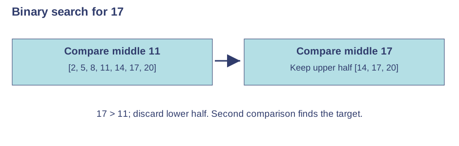
Use the labels alongside the associated explanation. - Choosing a search — A short unsorted list may suit linear search. A large already sorted list queried frequently benefits from binary search's repeated halving. Describe the method and constraints rather than asserting binary search is always best for every data set.
Sorting
- Bubble sort — An ascending bubble sort passes along the list comparing adjacent items. Larger items move towards the end. Repeated passes complete the order; a pass with no swaps can terminate early. Do not swap non-adjacent elements and call it a bubble-sort step.
Python bubble-sort recognition def bubble_sort(values): result = values.copy() for end in range(len(result) - 1, 0, -1): swapped = False for i in range(end): if result[i] > result[i + 1]: result[i], result[i + 1] = result[i + 1], result[i] swapped = True if not swapped: break return result print(bubble_sort([5, 2, 4, 1]))Outputs [1, 2, 4, 5]. Identify adjacent comparisons, the shrinking end and early termination; memorising this code is not required.
- Bubble-sort trace — For [5, 2, 4, 1], compare 5 and 2 to get [2, 5, 4, 1], then 5 and 4 to get [2, 4, 5, 1], then 5 and 1 to get [2, 4, 1, 5]. The largest is placed but further passes are needed.
- Insertion sort — Treat the first item as a sorted prefix. Take the next item and shift larger prefix items to make its correct place, then extend the prefix. For [4, 2, 3], inserting 2 gives [2, 4, 3], then inserting 3 gives [2, 3, 4].
Python insertion-sort recognition def insertion_sort(values): result = values.copy() for i in range(1, len(result)): item = result[i] j = i - 1 while j >= 0 and result[j] > item: result[j + 1] = result[j] j = j - 1 result[j + 1] = item return result print(insertion_sort([4, 2, 3]))Outputs [2, 3, 4]. Trace the sorted prefix and shifted items; memorising this code is not required.
- Merge sort — Divide the list into smaller parts until individual items remain, then merge ordered parts by repeatedly taking the smaller front item. Merge [2, 7] and [3, 5] as [2, 3, 5, 7]. The comparison is between the current fronts, not arbitrary pairs.
Python merge-sort recognition def merge_sort(values): if len(values) <= 1: return values.copy() middle = len(values) // 2 left = merge_sort(values[:middle]) right = merge_sort(values[middle:]) result = [] i = 0 j = 0 while i < len(left) and j < len(right): if left[i] <= right[j]: result.append(left[i]) i = i + 1 else: result.append(right[j]) j = j + 1 return result + left[i:] + right[j:] print(merge_sort([7, 2, 5, 3]))Outputs [2, 3, 5, 7]. Recursive calls divide the list; merge chooses from ordered fronts. Recognise the stages rather than memorising recursion.
- Comparing sorts — Bubble and insertion sorts are straightforward to trace; insertion can work well on nearly ordered lists. Merge sort's divide-and-merge approach suits larger data sets but needs additional working storage in common implementations. J277 requires understanding and applying the named methods, not formal complexity notation.
- Algorithm practice — Design a largest-value or validated-total algorithm, trace normal and boundary inputs, then correct a deliberate error. Use OCR Exam Reference Language or a familiar high-level language for code-writing tasks. Quick answers support this work but cannot replace constructing and checking a whole algorithm.